7-6. Add more continuous constraints
Repeat the pattern from 7-5 for four more constraint layers. Each one is a separate COG, prepared on the same grid as the wind power data.
For each row below: Add constraint → Direct URL → paste the URL → set the label, type Continuous, min, max and units → Save.
Slope — min 0, max 65, units degrees
https://eox-gtif-public.s3.eu-central-1.amazonaws.com/DHI/Copernicus_10m_DSM_COG_Slope_3857_fix.tif
Ruggedness Index — min 0, max 1, units index values
https://eox-gtif-public.s3.eu-central-1.amazonaws.com/DHI/RuggednessIndex_Austria_3857_COG_fix.tif
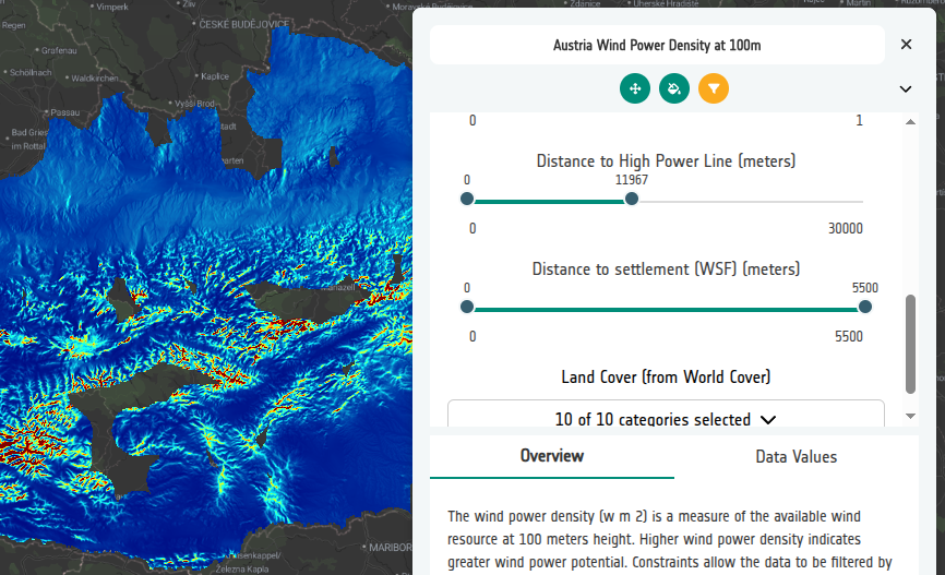
Distance to High Power Line — min 0, max 30000, units meters
https://eox-gtif-public.s3.eu-central-1.amazonaws.com/DHI/PowerLineHigh_EucDist_Austria_3857_COG_fix.tif
Distance to settlement (WSF) — min 0, max 5500, units meters
https://eox-gtif-public.s3.eu-central-1.amazonaws.com/DHI/WSF_EucDist_Austria_3857_COG_fix.tif
Combining constraints
Constraints are applied together: a pixel is only drawn where every active constraint is satisfied. That turns the layer into a simple site-suitability tool.
In the Preview, try narrowing several constraints at once:
- Land Cover — Cropland and Grassland only
- Elevation — below about 1500 m
- Slope — below about 15 degrees
- Distance to High Power Line — below about 5000 m
- Distance to settlement (WSF) — above about 1000 m
What remains is the accessible, buildable, grid-connected, non-residential land with the best wind resource.
Order matters for readability, not for logic
Constraints are combined regardless of their order in the list, but the order in the Constraints tab is the order they appear in the viewer. Use the move controls to put the most important filters first.