7-3. Add the wind power layer¶

Before adding constraints we need something to constrain. In this step we build a single COG layer showing wind power density at 100 m over Austria.

In the Layers tab, add a new Interface Group called Energy, then Add layer inside it and name the layer Austria Wind Power Density at 100m.

Add a COG data source with this URL:

https://eox-gtif-public.s3.eu-central-1.amazonaws.com/DHI/PowerDensity_100m_Austria_WGS84_COG_clipped_3857_fix.tif

Open Data Visualisation → Colormaps → Edit and add a colormap:

Setting Value

Name jet

Min 0

Max 2000

Steps 50

Reverse off
In the layer card Controls, enable:
- Opacity slider
- Zoom to centre
- Constraint slider
Leave Temporal controls and Blend controls off.

Constraint slider

Without the Constraint slider control the constraints you add in the following steps will be saved to the configuration but will never appear in the viewer.
Optional — polish the layer and the start location.

In the layer Metadata, set:
- Description — copy in the following text:
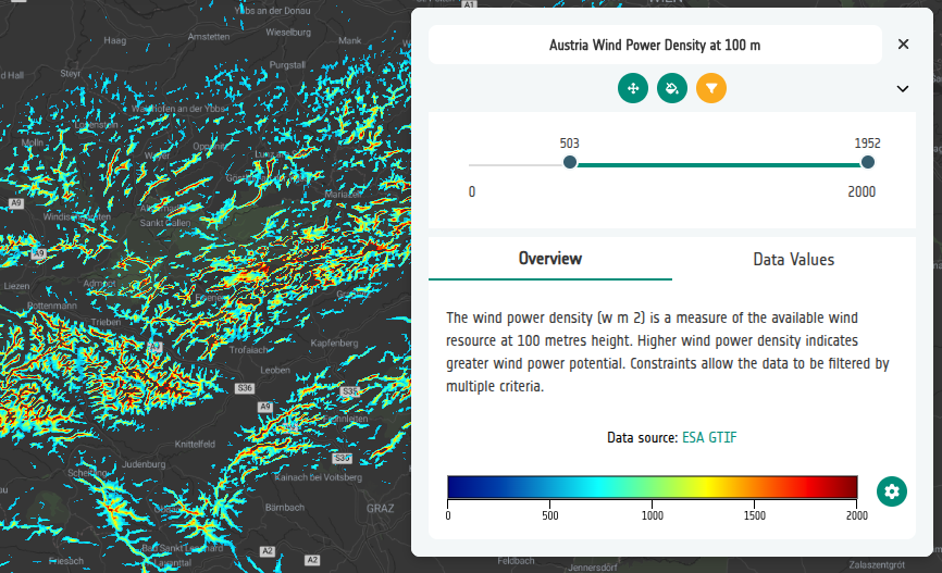
```
The wind power density (w m 2) is a measure of the available wind
resource at 100 metres height. Higher wind power density indicates
greater wind power potential. Constraints allow the data to be filtered
by multiple criteria.
```
- Units — w / m 2
- Attribution — text ESA GTIF, URL https://gtif.esa.int/
Then open Settings → Navigation and pick Austria from the quick location list, so the Explorer always opens on the area of interest. See 4-4. Default start location.
Open the Preview and turn the layer on. You should see a jet colour ramp over Austria with a gradient legend, and a Filter icon in the layer card. The filter is the constraint control for this layer: it lets you mask the wind power layer by its own data values, even before any additional constraint layers are added in the later steps.