7-5. Add a continuous constraint

The principle

A continuous constraint works on a variable that spans a full numeric range — elevation, slope, distance, temperature. Instead of checkboxes the viewer renders a two-handled slider, and the layer is only drawn where the constraint value falls between the two handles.

Here we constrain the wind power density by elevation, using a Copernicus DSM that has been prepared to match the wind power grid.

Configure it

1. In the Constraints tab of the Austria Wind Power Density at 100m layer card, select Add constraint.

2. Keep the source type as Direct URL and paste:

   https://eox-gtif-public.s3.eu-central-1.amazonaws.com/DHI/Copernicus_DSM_COG_10m_3857_fix.tif
   

3. Set:

   • Label — Elevation
   • Interactive — on
   • Constraint Type — Continuous

4. Select Populate Min & Max from COG. The builder reads the statistics from the file and fills in the range.

5. Round the values to 0 and 4000 so the slider has sensible stops, and set Units to meters.

6. Save the constraint.

View the result

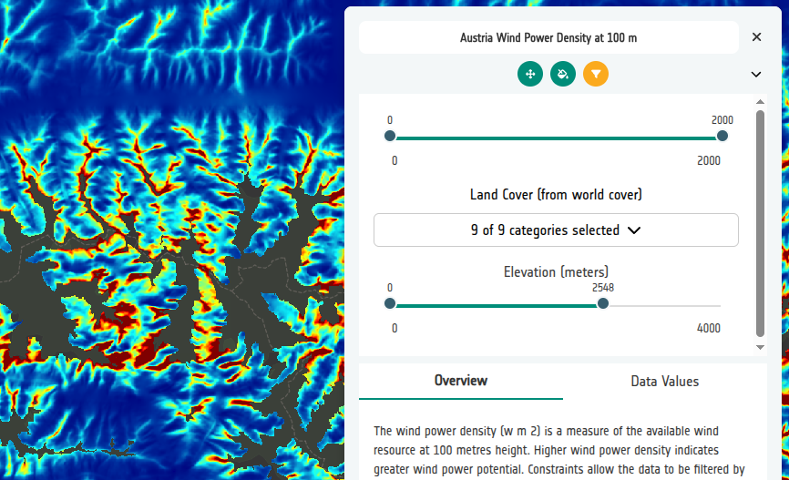
Open the Preview and drag the Elevation slider. As you pull the upper handle down, the high alpine areas drop out of the layer — useful, because the strongest modelled winds are often on summits where a turbine could never be built or connected.

Units matter

The units string is shown next to the slider values in the viewer. Without it a user has no way to know whether 4000 means metres or feet.

Did you remember to export?