11-4. Defining a custom CRS
The Geospatial Explorer ships with a set of built-in CRS options as noted in 11-2, but you are not limited to them. In this tutorial you will add EPSG:27700 — British National Grid as a custom CRS, use it as the display CRS for the map, and add a Sentinel-2 dataset that is supplied in OSGB so it lines up natively with the National Grid.
Defining the custom CRS
-
Start with either a new config, or add to your existing one from the earlier exercises.
-
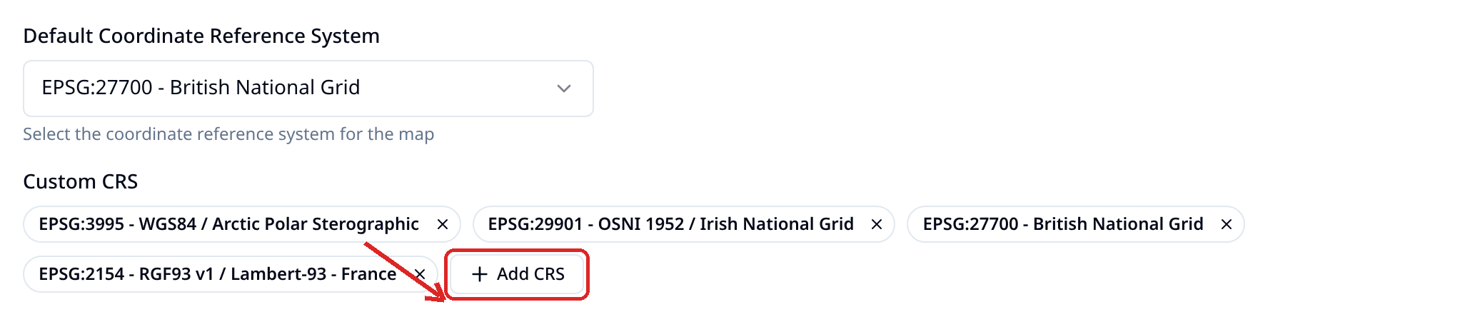
Open the Settings tab and scroll to the CRS section. Under Custom CRS, select + Add CRS and complete the dialog:
- Name:
British National Grid - CRS Code:
EPSG:27700 - PROJ.4 Definition:
+proj=tmerc +lat_0=49 +lon_0=-2 +k=0.9996012717 +x_0=400000 +y_0=-100000 +ellps=airy +units=m +no_defs +type=crs
The new CRS appears as a pill under Custom CRS and, from now on, in the Default Coordinate Reference System dropdown under Custom Projections.
- Name:
-
Set the Default Coordinate Reference System to EPSG:27700 - British National Grid.
-
Still in Settings, set the start location to the UK. In the Navigation section, choose United Kingdom from the Quick location list.
-
Open Preview. The map should now open on the UK in British National Grid rather than Web Mercator. If you zoom out a few times you will notice how data for the rest of the world now looks very different. This is because this CRS is optimised for minimising reprojection distortion in the UK and isn't concerned with data elsewhere!
Adding data that uses the custom CRS (optional)
We will now add some source data in this CRS. The following layer is stored in EPSG:27700.
-
Go back to the Layers tab and add a new layer called Sentinel 2 British National Grid. Choose + Add dataset → Direct Connection → COG and paste in this URL:
https://dap.ceda.ac.uk/neodc/sentinel_ard/data/sentinel_2/2026/09/21/S2A_20260921_latn518lone0007_T30UYC_ORB094_20260921161450_utm30n_osgb_vmsk_sharp_rad_srefdem_stdsref.tifClick on the (i) icon on the dataset row to view the metadata for the COG and note the EPSG it is in.
-
Define how to visualise the data. Select the pencil icon on Data visualisation → RGB composites. This will add the first 3 bands of this COG into the Red, Blue and Green channels. Select Save.
Info
Note the purpose of this exercise is to work with Coordinate Reference Systems, not visualisation. This step has not configured Sentinel 2 RGB bands onto these channels so the data will look a bit odd in the next step.
-
Open the Preview and toggle the newly added layer on.
-
Optionally, go to Settings -> CRS -> Default Coordinate Reference System and change back to EPSG:3857, then Preview again and toggle the layer on. You will notice that the data renders fine, although maybe slightly slower. This illustrates that this dataset is being reprojected on the fly from EPSG:27700 (our custom CRS) to Web Mercator. If you deleted the Custom CRS definition you would see that this data no longer renders.
Tip
PROJ.4 definitions for almost any CRS can be copied from https://epsg.io — search for the EPSG code and copy the PROJ.4 definition.