5-3. Categories for a COG
The category system determines how COGs are rendered when their values represent a data classification (as opposed to a continuous variable).
- Create a new layer card called
World Cover - Austriain the Land Cover interface group - see tutorial 2-6 for a recap if needed -
Add the following dataset — a World Cover COG for Austria - see tutorial 2-7 for a recap if needed:
https://esa-apex.s3.eu-west-1.amazonaws.com/APEX-example-data/constraints/PowerDensity_100m_Austria_WGS84_COG_clipped_3857_fix-esa_worldcover_2021.tif -
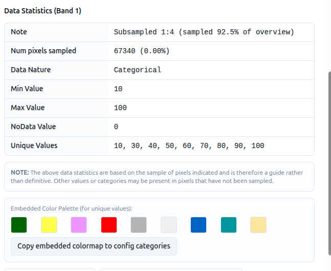
Click the (i) info icon on the dataset row to open the COG metadata dialog.
-
Use one of the category buttons to populate the editor:
- Populate categories (or Copy unique values to config categories) adds the classes found in the COG sample to the config, assigning arbitrary colours automatically. This is the fallback when a COG does not have an embedded colour map.
- Copy embedded colormap to config categories copies both the class values and their original colours from the COG itself. Use this option when the COG has an embedded colour map — this is the case for the World Cover Austria COG, so it is the preferred option here.
-
Edit a couple of the category labels to align to the World Cover class names (e.g.
10 → Tree cover,30 → Grassland). See the WorldCover class lookup below for the full list of values, colours and names.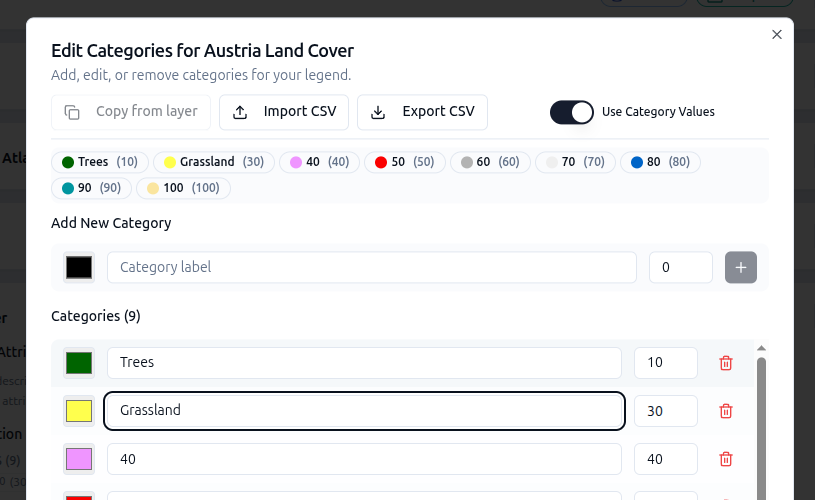
To save on manual typing you can also import or export categories from CSV files. If you want to do this quickly, download
world-cover-classes.csvand then import it from there. -
Save the layer card and preview. The COG is now rendered with the labels and colours you defined.
The values are populated from a sample of pixels. It is possible for a small number of pixels to fall into classes that were not sampled. Cross-check against the source data if completeness matters.
-
(Optional) Go back to Data Visualisation → Categories → Edit and change the colour of one class — for example, make Tree cover a light green. Save the layer card and preview again. The configured colour overrides the colour map embedded in the COG, so the legend and map rendering reflect your choice rather than the built-in palette.
WorldCover class lookup
| Value | Colour | Colour code | Class name |
|---|---|---|---|
| 10 | #006400 |
Tree cover | |
| 20 | #ffbb22 |
Shrubland | |
| 30 | #ffff4c |
Grassland | |
| 40 | #f096ff |
Cropland | |
| 50 | #fa0000 |
Built up | |
| 60 | #b4b4b4 |
Bare / sparse vegetation | |
| 70 | #f0f0f0 |
Snow and ice | |
| 80 | #0032c8 |
Permanent water bodies | |
| 90 | #0096a0 |
Herbaceous wetland | |
| 95 | #00cf75 |
Mangroves | |
| 100 | #fae6a0 |
Moss and lichen | |
| 0 | No data |