9-3. Styling multi-spectral data as natural colour
In this exercise we will work with an existing configuration. If you are following on from previous exercises you may want to export your current config, as we will load up a new one.
-
From the configuration builder Home page, select Load -> Tutorials -> Tutorial 9 pre-requisites.
About this config
This config file has a few multi-spectral datasets already included. Some of these are from the UK Earth Observation Data Hub so we have also added in support in this config for British National Grid as a custom Coordinate Reference System. Custom CRS definitions are covered in Tutorial 11 if you wish to replicate this elsewhere.
-
Take a look at the Bristol Sentinel 2 scene layer in the Sentinel 2 interface group. Right now this is just a normal layer, with a COG added, as you have done before.
- Note how the row in the Datasets tab tells us it has 10 bands, but they are "undefined".
- Now click on the ( i ) icon on that row to inspect the COG metadata. Note how it has a dropdown of bands and you can inspect the statistics of each individually.

-
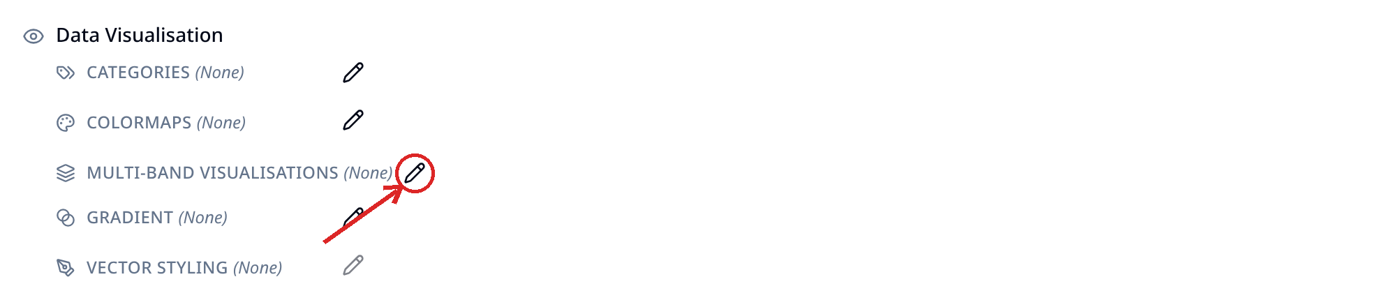
Now let's add some styling. On the main layer card select the Pen icon next to the multi-band visualisations option. This will open a popup with two tabs, one called Composites and another called Indices. Take a brief look at what is in each.
Composites vs indices. What's the difference?
Composites take three bands and visualise them in the red, green and blue channels of the output. If the input bands are also red, green and blue wavelengths, then this will look like a natural colour image. However, if they are other wavelengths then they will reveal patterns not visible to the naked eye.
Indices, meanwhile, make per-pixel calculations across multiple bands, ending up with a value typically between -1 and +1. These indices reveal interesting insights according to the formula used!
-
Select Composites -> Natural colour. You will see down the left that some bands have already been selected for you. You will also see some histograms. We will go with these defaults for now. Save the visualisation, and then go to Preview to take a look at the layer so far, zooming in to take a look in more detail.
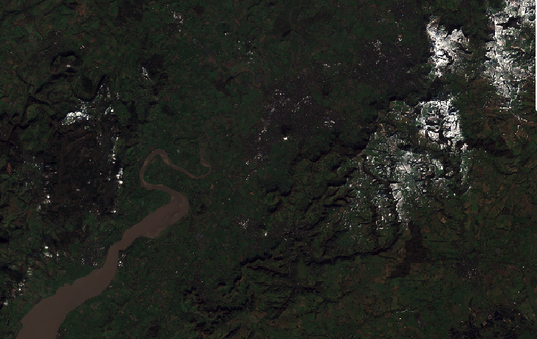
You might think the image looks a bit dark?
The natural colour visualisation you selected by default stretches the red, green and blue channels between 2 and 98% - i.e. ignoring 2% of pixels that are either really dark or really bright, to remove some outliers. However, you will have noticed that this scene, which is from January, includes areas of white - snow on the hills. This therefore means that a lot of bright pixels are influencing the stretch on the scene.
-
Return to the layer card, and edit the visualisation again (via the pen icon next to multi-band visualisation)! This time, apply the Mean +- σ stretch (where σ is standard deviation). Click save, then Preview and see how this has impacted the colour balance of the image.
